GPU SPH

About Smoothed Particle Hydrodynamics

The objective of this exercise was to use a combination of CUDA kernels to complete a larger task. To do so, I had to introduce synchronisation points, resolve conflicts for common memory addresses, and build optimisation structures.

Spatial data structure

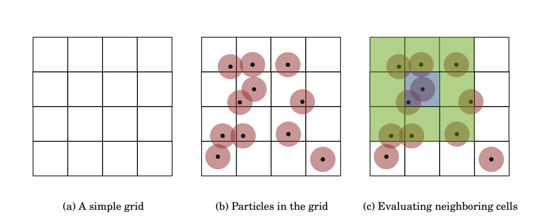
While it would be possible to test all pairs of particles for influences, it is not very efficient. The O(n²) complexity of this approach makes it very slow for higher particle counts. To speed up the detection process, a spatial data structure is usually used. Instead of testing all possible pairs, each particle is first inserted into the spatial data structure, which then provides a way to quickly find only the particles that currently reside within a particular region.

We used a simple, uniform grid data structure, built in four steps:

• Launch a kernel for each particle. Compute the grid cell the particle is currently in, and use atomicAdd to count the number of particles in each cell (cellCount).
• Run a prefix sum (scan) on cellCount to get memory offsets for each cell.
• Launch another kernel similar to the first, again using atomicAdd for counting the particles in each cell. Use the return value of the atomic operation to determine the particle's position within the cell. Combine this offset with the offset from the prefix sum to get the index in a global array grid.
• Launch a kernel for each particle. Again compute the particle's cell, look up the memory offset for this cell from the prefix sum result, and iterate through all particles in the same cell to determine possible collisions. As particles can be at cell boundaries and thus reach into neighbouring cells, extend the search to all 26 neighbouring cells.

The Navier-Stokes equation

Smoothed particle hydrodynamics builds upon the Navier-Stokes equation, which looks as follows:

where v is the velocity, p is the pressure, μ is the viscosity, f_ext are external forces, for example due to gravity, and ρ_m is the mass density, defined as ρ_m = m, where m is the mass.

SPH approaches the numerical integration of the Navier-Stokes equation by the simulation of particles. Each particle represents a sample in the space that is being simulated, and carries fluid properties such as mass, velocity, density and temperature. For our simulation, we associate each particle with a constant mass; we do not simulate temperature or more complex properties.

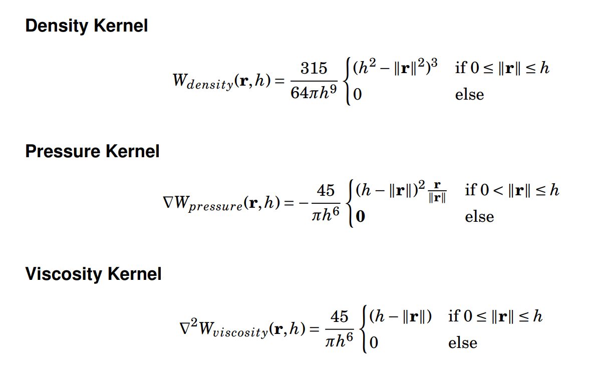
It must be possible to reconstruct the fluid properties for the entire space from the simulated particles. To this aim, the particle properties are smoothed out using a smoothing function W(r,h). The kernel support h can be seen as the area of influence, and r denotes the positional difference between two particles. In this exercise we use three smoothing kernels for the SPH simulation, with kernel support h equal to four times the particle radius:

To solve the Navier-Stokes equation it is necessary to compute the acceleration a particle experiences at a given time step (dv/dt), and to update the particle's position accordingly, considering the influence of (v * ∇)v. To this aim we have to compute the acceleration for each particle as defined on the right-hand side of the equation, which we achieve in five passes:

• Compute the density ρ for each particle.
• Calculate the internal pressure forces f_pressure from the densities.
• Compute the internal viscosity forces f_viscosity and the dissipation forces f_dissipation.
• Compute the external forces: gravity f_gravity and buoyancy f_buoyancy.
• Resolve collisions with obstacles.

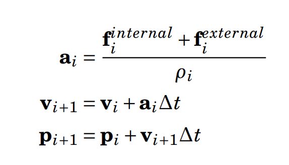
Then we can perform the integration step using semi-implicit Euler integration:

The individual forces

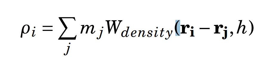
Density. Computing the density ρ_i for each particle location r_i is straightforward:

where j runs over all particles. Since the kernels are 0 for ||r_i - r_j|| > h, we only need to consider particles that are at most h away from particle i. The spatial data structure described above limits the computations to those particles. The density has to be computed in a separate kernel launch beforehand, since particles require the surrounding density for further computations.

Pressure. The pressure p can be derived from the density ρ as p = k(ρ - ρ₀), where k is a spring constant that defines how compressible a fluid behaves, and ρ₀ is the natural density of the fluid, the density at which no pressure arises. Ideally we would like a high k (ideally the square of the speed of sound), but that easily leads to instabilities as it would require very small time steps. In practice we have to work with a lower k.

To compute the pressure gradients it is necessary to estimate the pressure difference between all influencing particle pairs, which can be done using the symmetric difference estimator. This results in the following formula for the velocity change due to pressure:

Viscosity and dissipation. Viscosity can simply be modelled as particles transferring their velocity v to surrounding particles:

where μ is the viscosity coefficient of the fluid.

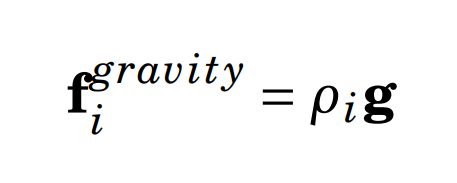
Gravity and buoyancy. Fluid particles experience a body force due to gravity g:

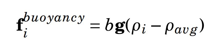
Buoyancy is an upward force opposing gravity, based on density differences inside the fluid. Depending on the fluid that surrounds a particle, the particle can either be dragged down or be spilled up. This behaviour can be modelled using the particle densities:

where b is the buoyancy coefficient and ρ_avg is the average surrounding density, computed by averaging the density values of all particles which lie within the kernel support h of the current particle.

And yep. If you got to here, your head probably just exploded like mine did when I first saw all of this. It was very hard and easy at the same time to implement: hard because one little accident in the formulas and nothing worked any more, and easy because all the equations were given and explained. In the end I got a great result.